Bayesian networks and causality
Correlation does not imply causality—you’ve heard it a thousand times. But causality does imply correlation. Being good Bayesians, we should know how to turn a statement like that around and find a way to infer causality from correlation.
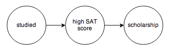
The tool we’re going to use to do this is called a probabilistic graphical model. A PGM is a graph that encodes the causal relationships between events. For example, you might construct this graph to model a chain of causes resulting in someone getting a college scholarship:
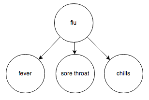
Or the relationship between diseases and their symptoms:
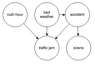
Or the events surrounding a traffic jam:
Each node represents a random variable, and the arrows represent dependence relations between them. You can think of a node with incoming arrows as a probability distribution parameterized on some set of inputs; in other words, a function from some set of inputs to a probability distribution.
PGMs with directed edges and no cycles are specifically called Bayesian networks, and that’s the kind of PGM I’m going to focus on.
It’s easy to translate a Bayesian network into code using this toy probability library. All we need are the observed frequencies for each node and its inputs. Let’s try the traffic jam graph. I’ll make up some numbers and we’ll see how it works.
Let’s start with the nodes with no incoming arrows.
val rushHour: Distribution[Boolean] = tf(0.2)
val badWeather: Distribution[Boolean] = tf(0.05)
In this hypothetical world, 20% of the time it’s rush hour, and 5% of the time there’s bad weather.
For nodes with incoming arrows, we return a different distribution depending on the particular value its in-neighbor takes.
def accident(badWeather: Boolean): Distribution[Boolean] = {
  badWeather match {
    case true => tf(0.3)
    case false => tf(0.1)
  }
}
If the weather is bad, we’re 30% likely to see an accident, but otherwise accidents occur only 10% of the time.
def sirens(accident: Boolean): Distribution[Boolean] = {
  accident match {
    case true => tf(0.9)
    case false => tf(0.2)
  }
}
Straightforward enough.
Now let’s tackle trafficJam. It’s going to have 3 Boolean inputs, and we’ll need
to return a different probabilty distribution depending on which of the inputs are true. Let’s say that
if any two of of the inputs are true, there’s a 95% chance of a traffic jam, and that
traffic jams are less likely if only one of them is true, and somewhat unlikely if none are.
def trafficJam(rushHour: Boolean,
               badWeather: Boolean,
               accident: Boolean): Distribution[Boolean] = {
  (rushHour, badWeather, accident) match {
    case (true, true, _) => tf(0.95)
    case (true, _, true) => tf(0.95)
    case (_, true, true) => tf(0.95)
    case (true, false, false) => tf(0.5)
    case (false, true, false) => tf(0.3)
    case (false, false, true) => tf(0.6)
    case (false, false, false) => tf(0.1)
  }
}
If you’ve done any Scala or Haskell programming, you’ve probably noticed that these are all functions of type
A => Distribution[B]—and yeah, you better believe we’re gonna flatMap that shit.
So let’s wire everything up and produce the joint probability distribution for all these events.
case class Traffic(
  rushHour: Boolean,
  badWeather: Boolean,
  accident: Boolean,
  sirens: Boolean,
  trafficJam: Boolean)

val traffic: Distribution[Traffic] = for {
  r <- rushHour
  w <- badWeather
  a <- accident(w)
  s <- sirens(a)
  t <- trafficJam(r, w, a)
} yield Traffic(r, w, a, s, t)
Now we can query this distribution to see what affects what.
Say you’re about to head home from work and you notice it’s raining pretty hard. What’s the chance there’s a traffic jam?
scala> traffic.given(_.badWeather).pr(_.trafficJam)
res0: Double = 0.5658
Then you hear sirens.
scala> traffic.given(_.badWeather).given(_.sirens).pr(_.trafficJam)
res1: Double = 0.6718
About what you’d expect. Sirens increases your belief that there’s an accident, which will in turn affect the traffic.
Let’s look at things the other way around. Say you’re sitting in traffic and you want to know whether there’s an accident up ahead.
scala> traffic.given(_.trafficJam).pr(_.accident)
res2: Double = 0.3183
Also, it’s raining, so you decide to factor that in:
scala> traffic.given(_.trafficJam).given(_.badWeather).pr(_.accident)
res3: Double = 0.4912
Makes sense, bad weather increases the chance of an accident.
Suppose instead the weather is fine, but it is rush hour:
scala> traffic.given(_.trafficJam).given(_.rushHour).pr(_.accident)
res4: Double = 0.1807
That’s interesting, adding the knowledge that it’s rush hour made the likelihood that there’s an accident go down. But there’s no direct causal link in our model between rush hour and accidents. What’s going on?
Belief propagation
The neat thing about Bayesian networks is that they completely explain which nodes can be correlated and which are independent. By following a few simple rules, you can read this information right off the graph.
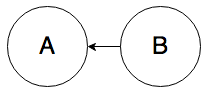
Rule 0. In the graph below, A and B can be correlated:
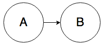
It’s almost too simple to mention, but knowing the value of A will change your belief about the value of B.
What’s slightly less obvious is that knowing the value of B will change your belief about the value of A. For example, if rain causes the sidewalk to be wet, then seeing a wet sidewalk changes your belief about whether it rained.
Rule 1. In the graph below, A and B can be correlated:
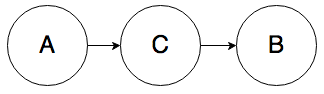
Knowing the value of A will change your belief about the value of B. Furthermore, knowing the value of B will also change your belief about the value of A. Intuitively, if someone got a scholarship (B), that raises your belief about whether they studied for their SATs (A), even if there’s an intermediate cause in the mix, say a high SAT score (C).
So far, it seems like belief can propagate through arrows in either direction.
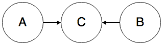
Rule 2. In the graph below, A and B can be correlated:
Knowing the value of A influences your belief about the value of C, which directly affects the value of B. For example, knowing that someone has a fever (A) increases your belief that they have the flu (C), which in turn increases your belief that they have a sore throat (B).
So what’s the point of arrows if belief can propagate across them in either direction? Glad you asked.
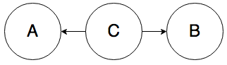
Rule 3. In the graph below, A and B must be independent:
To give you the intuition, whether the weather is bad (A) should have no influence over whether it’s currently rush hour (B), even though they both cause traffic jams (C).
So we have two cases where belief can propagate through a node, and one case where it can’t. But something interesting happens when the value of the middle node, C, is known—the situation completely reverses.
Belief propagation with observed nodes
Rule 1a. In the graph below, if C is known, A and B must be independent.
Knowing C “blocks” belief from propagating from A to B. If you know that someone got a high SAT score (C), whether they studied for their SATs (A) doesn’t tell you anything new about whether they got a scholarship (B). In the reverse case, if you know that someone got a high SAT score, then knowing whether or not they got a scholarship should not change your belief about whether or not they studied.
Rule 2a. In the graph below, if C is known, A and B must be independent.

Again, knowledge of the middle node blocks belief from propagating through it. If you know someone has the flu (C), knowing that they have a sore throat (A) does not affect your belief that they have a fever (B); knowing that they have the flu already tells you everything you need to know about their body temperature.
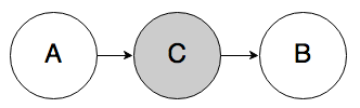
Rule 3a. In the graph below, if C is known, A and B can be correlated.
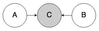
This case is interesting—normally, belief would not be able to propagate through node C like this, but if its value is known, the node becomes “activated” and belief can flow through. The intuition here is that if I already know that there’s a traffic jam (C), then knowing that it’s rush hour (A) should decrease my belief that the weather is bad (B). Rush hour “explains away” the traffic jam, making bad weather seem less likely.
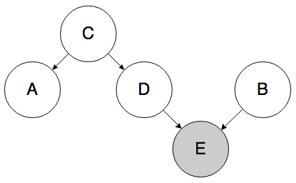
Rule 3b. In the graph below, if D is known, A and B can be correlated.
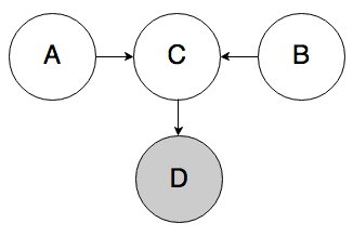
This rule is a variation on Rule 3a. If we know D, then we also know something about C, which partially activates C and allows belief to flow through it from A to B. For example, if I observe someone wearing a college sweatshirt (D), that increases my belief that they went to college (C). If I find out that they got a high SAT score (A), that can decrease my belief that they played sports (B).
These rules are collectively known as the Bayes-Ball algorithm. There’s no Dr. Ball; it’s just a pun on “baseball.” Statistics jokes: they’re probably funny!
Anyway, now that we have some rules, let’s put them to use.
Are coin flips independent?
Everyone knows that coin flips are independent of one another—if you flip a fair coin 10 times and it comes up heads each time, the probability that it will come up heads on the next flip is stil 50%.
But here’s a different argument: If I flip a coin 100 times and it comes up heads 85 times, I might notice that this is astronomically unlikely under the assumption that I have a fair coin, and call shenanigans on the whole thing. I could then reasonably conclude that the coin’s bias is actually 85%, in which case the next flip is maybe 85% likely to come up heads—meaning the next flip was not independent of the other flips!
How can we reconcile these two arguments? There’s a subtle difference between the two that becomes clear when you draw out the graph.
Here’s the first case:
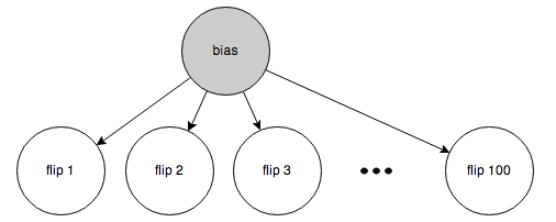
The bias is known (50%), so belief is blocked from propagating between the individual flips (Rule 2a).
Here’s the second case:
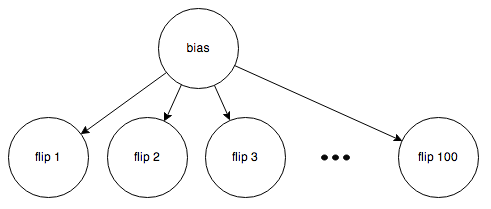
Here, the bias is unknown, so belief is allowed to flow through the “bias” node (Rule 2).
So both are right! They just make subtly different assumptions.
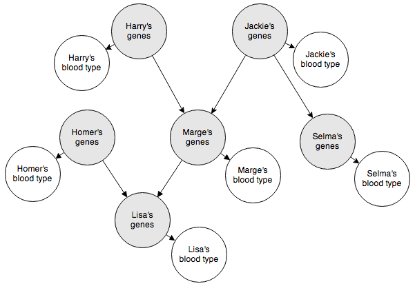
Reasoning about hidden nodes
The Bayesian network below represents the blood types of several members of a family. The shaded nodes indicate nodes we can’t observe. But as long as we know how they interact with the observable nodes, we can make inferences about how the observable nodes interact with each other.
This will be pretty fun to code up. Here’s how we’ll represent the genotypes and phenotypes (blood types):
sealed trait BloodGene
case object A_ extends BloodGene
case object B_ extends BloodGene
case object O_ extends BloodGene

sealed trait BloodType
case object A extends BloodType
case object B extends BloodType
case object AB extends BloodType
case object O extends BloodType
Yeah, I know, Scala makes this unnecessarily verbose.
For the arrows linking each person’s genes to their blood type, we need a function that determines BloodType given
two BloodGenes. This happens to be a deterministic function, but I’m implementing it as a stochastic function anyway.
def typeFromGene(g: (BloodGene, BloodGene)): Distribution[BloodType] = {
  g match {
    case (A_, B_) => always(AB)
    case (B_, A_) => always(AB)
    case (A_, _) => always(A)
    case (_, A_) => always(A)
    case (B_, _) => always(B)
    case (_, B_) => always(B)
    case (O_, O_) => always(O)
  }
}
For the arrows linking parents’ genes to their children’s genes, we can implement this function that chooses one gene from each parent at random:
def childFromParents(p1: (BloodGene, BloodGene),
                     p2: (BloodGene, BloodGene)): Distribution[(BloodGene, BloodGene)] = {
  val (p1a, p1b) = p1
  val (p2a, p2b) = p2
  discreteUniform(for {
    p1 <- List(p1a, p1b)
    p2 <- List(p2a, p2b)
  } yield (p1, p2))
}
Finally, for the people whose parents are not specified, we supply a prior on each of the 3 genes refecting their prevalence in the general population.
val bloodGenePrior: Distribution[(BloodGene, BloodGene)] = {
  val geneFrequencies = discrete(A_ -> 0.26, B_ -> 0.08, O_ -> 0.66)
  for {
    g1 <- geneFrequencies
    g2 <- geneFrequencies
  } yield (g1, g2)
}
OK, now let’s wire everything up. This should be a straightforward translation of the Bayesian network above into code.
case class BloodTrial(lisa: BloodType, homer: BloodType, marge: BloodType,
                      selma: BloodType, jackie: BloodType, harry: BloodType)

val bloodType: Distribution[BloodTrial] = for {
  gHomer <- bloodGenePrior
  gHarry <- bloodGenePrior
  gJackie <- bloodGenePrior
  gSelma <- childFromParents(gHarry, gJackie)
  gMarge <- childFromParents(gHarry, gJackie)
  gLisa <- childFromParents(gHomer, gMarge)
  bLisa <- typeFromGene(gLisa)
  bHomer <- typeFromGene(gHomer)
  bMarge <- typeFromGene(gMarge)
  bSelma <- typeFromGene(gSelma)
  bJackie <- typeFromGene(gJackie)
  bHarry <- typeFromGene(gHarry)
} yield BloodTrial(bLisa, bHomer, bMarge, bSelma, bJackie, bHarry)
Here it is in action:
scala> bloodType.map(_.marge).hist
 A 40.40% ########################################
 B 11.19% ###########
AB  4.25% ####
 O 44.16% ############################################

scala> bloodType.given(_.lisa == B).map(_.marge).hist
 A 12.65% ############
 B 42.98% ##########################################
AB 13.32% #############
 O 31.05% ###############################

scala> bloodType.given(_.lisa == AB).map(_.marge).hist
 A 45.71% #############################################
 B 37.40% #####################################
AB 16.89% ################
Makes sense so far. Let’s look at Lisa and her Aunt Selma:
scala> bloodType.map(_.lisa).hist
 A 41.79% #########################################
 B 11.24% ###########
AB  3.94% ###
 O 43.03% ###########################################

scala> bloodType.given(_.selma == A).map(_.lisa).hist
 A 52.82% ####################################################
 B  7.47% #######
AB  4.90% ####
 O 34.81% ##################################

scala> bloodType.given(_.selma == B).map(_.lisa).hist
 A 26.84% ##########################
 B 27.22% ###########################
AB  9.08% #########
 O 36.86% ####################################
Homer and Marge should not affect each other, unless Lisa’s blood type is known:
scala> bloodType.map(_.homer).hist
 A 40.34% ########################################
 B 10.74% ##########
AB  4.21% ####
 O 44.71% ############################################

scala> bloodType.given(_.marge == A).map(_.homer).hist
 A 40.60% ########################################
 B 10.83% ##########
AB  3.91% ###
 O 44.66% ############################################

scala> bloodType.given(_.lisa == B).map(_.homer).hist
 A 11.91% ###########
 B 42.84% ##########################################
AB 13.77% #############
 O 31.48% ###############################

scala> bloodType.given(_.lisa == B).given(_.marge == A).map(_.homer).hist
 B 73.99% #########################################################################
AB 26.01% ##########################
This is Rule 3b in effect. Even Harry and Jackie are correlated if their grandchild’s blood type is known:
scala> bloodType.given(_.lisa == AB).map(_.harry).hist
 A 43.83% ###########################################
 B 23.51% #######################
AB 10.90% ##########
 O 21.76% #####################

scala> bloodType.given(_.lisa == AB).given(_.jackie == O).map(_.harry).hist
 A 45.01% #############################################
 B 37.73% #####################################
AB 17.26% #################
This is pretty fun to play around with!
Causal fallacies
If you observe that two events A and B are correlated, you cannot determine the direction of causality from observational data on these two events alone. Any of
(“A causes B”) or
(“B causes A”) or
(“A and B have a common cause”) could explain the observed correlation. But there’s also this possibility:
where C is known. This is just a biased sample—you might conclude that academic ability interferes with athletic ability after observing that they are inversely correlated, until you realize you only surveyed college students, and that academic and athletic scholorships are quite common. But it’s neat that graphical models unify these causal fallacies.
To go further, you could come up with crazy causal graphs that predict a correlation between A and B, but where the causal link between A and B is non-trivial. For example, the graph below allows A and B to be correlated, but neither directly causes the other, they don’t have a common cause, and although there is a biased sample, it appears to only directly affect B.
Determining causality
This brings up an important question: if I observe some events and their frequencies, how can I figure out which of the possible graphs I could draw is the correct one? Well, the great thing about Bayesian networks is that they make testable predictions. In particular, for a given graph, if the independence relations that we now know how to read off of it do not bear themselves out empirically, we can eliminate that graph as a possibility. We can also use common sense to rule out graphs that make unphysical predictions, for example, the sidewalk being wet causes it to rain, and effects preceding their causes in general.
To take an example, the graph
predicts that A and B are independent, unless C is known. If we observe that, say, , then we can rule out that graph as a possible model.
Usually we can use observations like this to narrow down the set of possible graphs. With only 2 events to observe, there’s no way to distinguish and just from the data. With 3 events that are all dependent, you can’t distinguish between and and . However, you can distinguish from , since in the first case, and are independent when you control for .
If you’re lucky, you can narrow down the set of possible graphs enough to be able to infer what arrows there are and what direction they point in. And before you know it, you’ve inferred causality from mere correlation. Voilà!
In practice, though, this rarely happens, especially if you have more than like 5 nodes in your graph. There are simply too many possible graphs to consider, and the very connected ones don’t make any predictions at all that might help us falsify them. But if you can step in and control things a bit, you can simplify the interactions and make the problem tractable again.
Controlled experiments
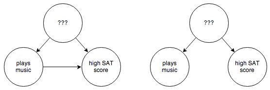
Suppose you’re trying to decide whether playing a musical instrument results in higher SAT scores. In your empirical observations you’re careful to identify socioeconomic status as a possible confounding factor. Say you end up with the following 2 possible graphs:
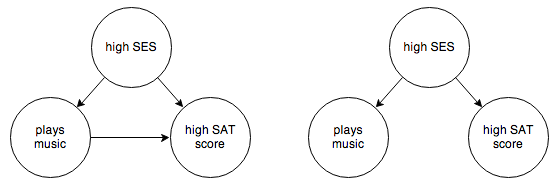
You want to know whether the arrow from “plays music” to “high SAT score” exists or not. One thing you can try is to control for socioeconomic status:
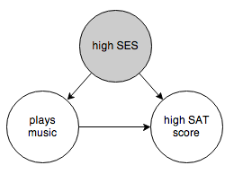
This prevents belief from propagating through the “high SES” node. If “plays music” and “high SAT score” are still correlated after controlling for socioeconomic status, then you can eliminate the graph on the right and conclude that there is a causal link between the two events. (Technically we don’t know which way the arrow should point, but that’s where common sense steps in.) If “plays music” and “high SAT score” are independent when controlling for socioeconomic status, then you have to reject the graph on the left and accept that there is no direct causal link between the events.
Socioeconomic status might not be the only confounding factor, though. There are a whole host of possible confounding factors, and we can’t rule out the possibility that we missed one. So what we really have is this:
You can’t control for things you can’t observe. So in this case you have to step in and rewire things a bit:
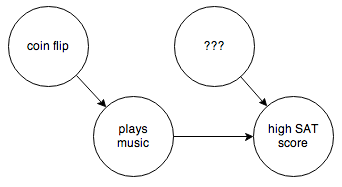
By forcing “plays music” to be determined randomly and independent of anything else, you break the causal link between it and any other confounding factors. Then it’s easy to determine whether the arrow between “plays music” and “high SAT score” really exists.
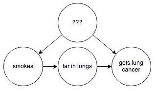
But often this is not practical. In an example cribbed from this excellent article on the subject, suppose you are trying to determine whether smoking causes lung cancer directly, or if instead there are some environmental factors that happen to cause both. You have the following possible graphs:
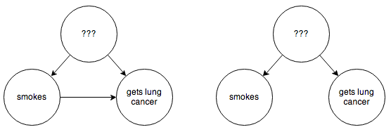
You can’t step in and force some people to smoke or not smoke. You’d think we might be stuck here, but fortunately some extremely clever people have figured out how to infer causality in a situation like this without needing to run a controlled experiment. In this example, if you are able to hypothesize some observable intermediate cause, such as the presence of tar in someone’s lungs:
then through a series of formal manipulations, you can arrive at a graph that, weirdly enough, looks like this:
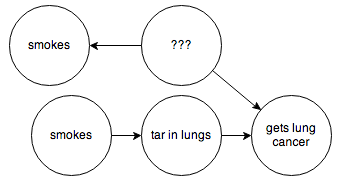
The two “smokes” nodes have the same probability distribution but are independent from one another.
This is pretty great! Using the “smokes” node on the bottom, we can now ask this graph about the probability of someone getting cancer, as if their decision to smoke was independent of any other factors. In other words, we can now determine what would have happened if we had been able to force our subjects to smoke or not smoke in a controlled experiment.
Before we do that, though, we’re going to need to make one more little change—as it is, we’re going to run into trouble with the “???” node. Since this node represents unknown causes in our model, we’re not going to be able to observe it or its effects on other nodes. Fortunately, due to the magic of the Bayes-Ball rules, we can replace it with an arrow that goes directly from “smokes” to “cancer”, without changing the meaning of the graph. So our two graphs become:
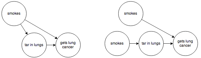
Now all of our nodes and arrows are observable, and we can go ahead and code this up.
Suppose we observe that 50% of the population smokes. We’ll have:
def smokes: Distribution[Boolean] = tf(0.5)We can also encode observations of the frequencies at which smokers and non-smokers have tar in their lungs:
def tar(smokes: Boolean): Distribution[Boolean] = {
  smokes match {
    case true => tf(0.95)
    case false => tf(0.05)
  }
}
And the last one, observed frequencies of cancer, broken out by whether someone smokes or has tar in their lungs:
def cancer(smokes: Boolean, tar: Boolean): Distribution[Boolean] = {
  (smokes, tar) match {
    case (false, false) => tf(0.1)
    case (true, false) => tf(0.9)
    case (false, true) => tf(0.05)
    case (true, true) => tf(0.85)
  }
}
Again, these numbers represent simple observed frequencies. We could actually do this in practice if we had experimental data. (Obviously all the numbers here are extrememly made up.)
Now let’s wire everything together. We’ll do it two ways: the first way encoding the original graph, and the second way encoding the manipulated graph that separates “smokes” from external influences.
case class SmokingTrial(smokes: Boolean, tar: Boolean, cancer: Boolean)

def smoking1: Distribution[SmokingTrial] = {
  for {
    s <- smokes
    t <- tar(s)
    c <- cancer(s, t)
  } yield SmokingTrial(s, t, c)
}

def smoking2: Distribution[SmokingTrial] = {
  for {
    s1 <- smokes
    s2 <- smokes
    t <- tar(s1)
    c <- cancer(s2, t)
  } yield SmokingTrial(s1, t, c)
}
Now let’s see it in action.
scala> smoking1.pr(_.cancer)
res0: Double = 0.4723

scala> smoking1.given(_.smokes).pr(_.cancer)
res1: Double = 0.8576

scala> smoking2.pr(_.cancer)
res2: Double = 0.4759

scala> smoking2.given(_.smokes).pr(_.cancer)
res3: Double = 0.4577
According to these made-up numbers, smoking actually prevents cancer, even though empirically, smokers have a higher incidence of cancer than the general population!
This is pretty miraculous, if you ask me.
Further reading
Less Wrong has a great introduction on using Bayesian newtworks and the predictions they make to determine the direction of causality.
Here are some slides from lectures on the Bayes-Ball algorithm and how a Bayesian network factors a joint probability distribution.
You should also read Michael Nielsen’s fantastic article explaining Judea Pearl’s work on simulating controlled experiments in, like, the nineties. This is cutting-edge stuff! I bet you thought all of probability was worked out in the 1700s!
I also recommend the Coursera on probabilistic graphical models.
All of the code in this post is available in this gist.
Thanks to Blake Shaw for his feedback on early drafts of this post.
blog comments powered by Disqus